JW Player introduced analytics as a major feature with JW6 in 2012. This allowed us to offer publishers insights into who was watching their content, including device, geo and video data. Adoption of JW6 exploded over the next 3 years, challenging us to keep up with the rapidly increasing data coming in each day. This article looks to explore a particular challenge we’ve faced in scaling our periodic batch pipeline for publisher analytics: key skew in Hadoop.
Issues scaling JW analytics
In May 2015, our publishers collectively reached 1.2 billion viewers watching 71k years of video. We receive multiple terabytes of raw data each day, plus many terabytes more of intermediate and final data we process in our various pipelines for publisher analytics, JW Trends and other projects. Keeping up with our growing publisher base and scaling our infrastructure is something we’ve worked hard on here at JW Player.
We operate many pipelines to process data with numerous components, each with its own issues in scaling. Some components scale easily, others scale problem free until we reach a critical point in our growth and issues become apparent. The rapid growth of JW Player 6 means we’re constantly evolving, improving and scaling our infrastructure.
Early on, after the release of JW6, a single large publisher coming online could comprise a large amount of our analytics data. Additionally, video level data accounted for an overwhelming amount of our final processed data, with our largest publishers embedding players with millions of unique video URLs each day. This informed our thinking of scale later on, though as we’ll see later in the article, we’ve had to update our thinking as our data grows and new problems emerge.
What Is Skew?
Processing large amounts of data often depends on the high parallelism of the tools and algorithms used. In other words, we can split the data and work into chunks that we can spread and share across machines in a cluster. This allows us to process more and more data, not just by increasing the raw computing power of the individual instances we use, but by also using more and more instances in our clusters, increasing our effective maximum computing power.
Skew is fundamentally about a skew in this parallelism, where it becomes increasingly difficult and time consuming to process growing amounts of data despite comparably growing our computing power. Instead of the data and workload being evenly shared across a cluster, certain individual components get an excessive amount of data or take an excessive amount of time to process its data.
Typically, these parallel processes require all components to finish before the next process can start. You end up with a situation where you have a large cluster mostly sitting idle while a small number of components continue crunching their share. This is obviously inefficient, but it also makes it difficult to scale your data processing. Adding more instances or computing power has limited benefit, especially compared to an even workload.
JW Analytics Pipeline
Before delving into the specifics of our skew issue, I’d like to explain a little about the relevant infrastructure. I’ll cover how we collect data from the players out in the wild and cover our periodic pipeline where we process a lot of our publisher and network analytics. I’ll also go into detail of the Crunch Logs step, which is the specific Hadoop job where our skew issue was.
Data Collection
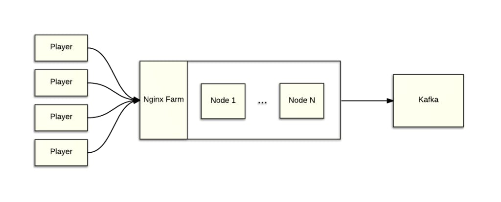
Our data collection system is relatively straightforward. The ping plugin in each player pings back data in the form of a request for a 1×1 GIF. These requests contain information about embeds, plays, engagement and other kinds of data. We use Nginx to serve and log these requests, which are then sent to a Kafka cluster for central storage and easy access by our various pipelines and systems.
Periodic Batch Pipeline
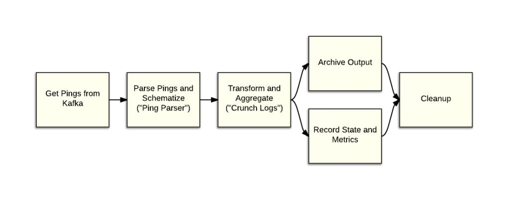
Here we see a slightly simplified diagram of our periodic batch pipeline where we do a lot of processing of publisher and network analytics. The periodic pipeline has the following major steps:
Get Pings from Kafka – Like all of our pipelines and other projects, Kafka is the central store for our ping data. Here we are pulling the Nginx request logs that contain the raw ping data.
Parse Pings and Schematize (“Ping Parser”) – In this step, we parse each log line and convert it into Avro. As part of the parsing, we do geo lookups, user agent parsing, and other processing.
Transform and Aggregate (“Crunch Logs”) – This is the problem step. To put it simply, this step transforms and aggregates the rich ping Avro objects into about 20 different slices of data. I’ll go into more detail in the next section.
Archive Output – We store the output on the Crunch Logs and Ping Parser steps in S3 for further processing and archival purposes
Record State and Metrics – Here we record state and metrics, such as Kafka offsets
Cleanup – At the end, we cleanup to prepare for the next run of the periodic
Crunch Logs in Detail
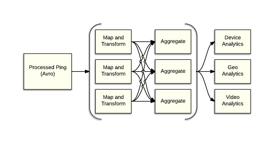
Finally, we’re at the problem step. Crunch Logs is a custom Hadoop job written in Java. We take ping Avro objects as input and output around 20 different Avro types that represent different slices of our data.
We use a mapping configuration file that tells Crunch Logs how to map, transform and aggregate the incoming pings. This mapping format supports a few basic transformation and aggregation functions (i.e. date parsing and counting distinct values), as well as limited filtering. This allows us to cut a bunch of slices in a single, efficient pass.
Skew Revisited
Now that we’ve gone through an overview of the relevant infrastructure, let’s dive into our skew problem. We’ll start with a basic explanation of Hadoop and how skew affects its performance, then move onto how skew affected us and how we eventually solved our problem.
Hadoop Primer
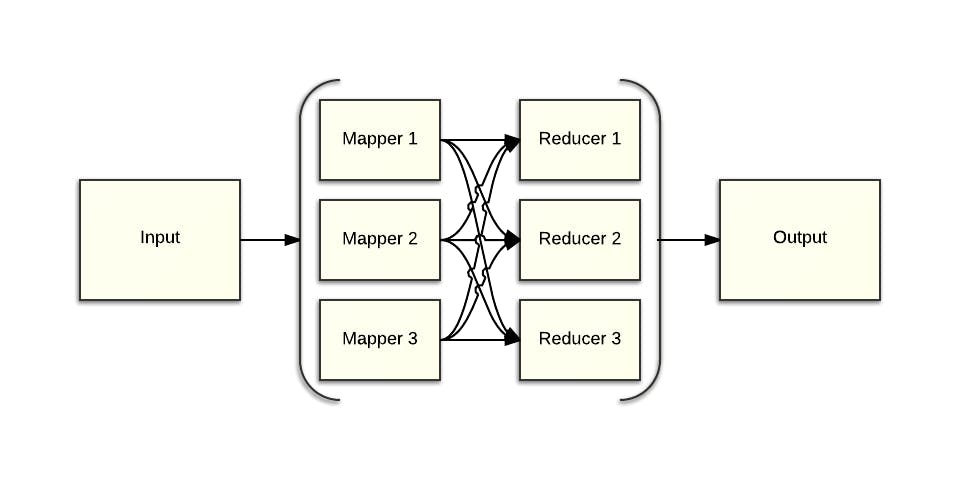
At its core, Hadoop is an implementation of the MapReduce programming model. What this allows us to do is build distributed, parallel and fault tolerant applications for processing large amounts of data within a standard framework.
At a high level, there are two major components: mappers and reducers. Input data is split between the mappers roughly evenly, which is typically easy, and can be text, pictures or any other type of data. The mappers then process their data; each input record is processed and then zero, one or more key/value pairs are outputted. The output for each mapper is partitioned between all of the reducers. By default, a hash of the key is used to determine which reducer gets which keys. This guarantees that all key/value pairs for the same key go to the same reducer.
The reducers can then perform calculations such as summing all values for a given key. Because of the above guarantee that all key/value pairs of a single key go to the same reducer, we can guarantee a global sum of all of the values of that key or guarantee a global count of all unique values for that key. If the values for a given key were split among two or more reducers, we couldn’t guarantee that property.
Skew in Hadoop
Guaranteeing input data is evenly split among the mappers is generally easy. If you have 3 mappers, you divide the input data in thirds. But guaranteeing equal loads for the reducers can be tricky. Skew happens when a subset of the reducers has a greater share of the load, causing the overall job to take longer than ideal. In the worst case, 1 reducer can be responsible for a large amount of the overall data, causing the job to take a long time and making it difficult to scale.
This happens when a relatively small number of keys are overrepresented in the mapper outputs. Remember, by default, Hadoop guarantees all instances of a given key go to the same reducer. If that key is vastly overrepresented, that reducer will take longer to run than it would under an even load.
Our original understanding
Our initial issues with scaling dealt with the rapid, exponential growth in adoption with JW6. The JW Player was extremely popular among both small sites and large publishers for a long time, and JW6 was no different. Additionally, the overall makeup of our network was rapidly changing.
Given this understanding, we wanted our solution to work along these lines:
Algorithmically determine which keys were skewed each run – Our rapidly growing and changing data would make the skew issue a moving target. We wanted to be able to adapt to a changing skew problem.
Maintain sending all instances of a given key to a single reducer – We wanted to maintain the property of having our aggregations being globally complete within each run
Make sure these skewed keys were distributed roughly evenly among reducers – We would evenly distribute the skewed keys across the reducers as best as we can.
We started by adding a job that would sample our data each run. This would allow us to find our top X skewed keys each run while minimizing added overhead. We then added a custom partitioner. If the key was in the list of skewed keys, we would partition the key to ensure it has little or no overlap with the other skewed keys. If the key was not in the list, it would be partitioned normally.
Unfortunately, this didn’t solve our problem.
Taking a step back
Over time, Crunch Logs grew increasingly time consuming in line with the growth in our data. Adding more instances reached severely diminishing returns. Additionally, our publisher base was large and diverse by this point. The biggest publishers, while sending lots of data to us, have a large number of keys in our data due to the many devices, countries, videos and other data that go into our publisher analytics. It’s doubtful we were seeing a publisher with enough overall volume that was all going into a single device, country or other key.
The performance we saw was consistent with having a very large and ever increasing amount of data in a small number of keys. Our various publisher level analytics didn’t appear to fit this. What could possibly fit this profile? This is when the light bulb goes off. It must be our high level network analytics! Large amount of data: check! Small number of keys in the aggregations: check! Explains the performance characteristics we’ve seen over the previous months: check! We now had our culprit, but how could we solve our problem?
Re-re-partitioning our data
Originally, we thought the skewed keys were a moving target, but in reality they were not. They came from a couple of network level slices of data, which meant they came from particular mappings. It also meant we couldn’t maintain the one key, one reducer guarantee. We had to spread those keys among multiple reducers.
It turned out that this wasn’t too big of an issue. The aggregations in the periodic are not global in our system. They were merely global for the chunk of data the batch process was working on. We had a separate daily process to perform a final aggregation on the data to guarantee a true global aggregation of the keys.
We added a partition type to the mapping configuration, which allowed us to specify the particular partition function we wanted to use for each slice of data. We added a random partitioner to split keys among a number of reducers randomly. This greatly reduced the run time and skew of our Crunch Logs step and lacked the overhead in our original solution.
Potential future improvements
Our solution worked well and was simple to implement. But it wasn’t without down sides. It requires prior knowledge of the data set and has to be manually set. You can also run into an issue where you can split those mappings across too many reducers, greatly adding to the number of files to be processed by the daily, which is its own performance issue.
Another solution we’ve discussed, but not implemented, is to do limited mapper side aggregation. Like our original plan, you can algorithmically determine and store the skew keys using an LRU map cache. While keys live in the map, you aggregate them. When they fall out, or when the mapper reaches the end of its input data, you write out the keys normally. This gives us back our one key/one reducer guarantee, while also not requiring us to manually determine our partitioning strategy.
Conclusion
It has been interesting to see the evolution of our thinking regarding this skew problem, not just from the point of view of the problem itself, but also in how we’ve understood our data makeup and size throughout the different components of our systems. It shows how our assumptions and previous understandings can lead us down wrong paths. And it underscores the importance of knowing when to take a step back and reevaluate what you thought you knew to be able to solve the problems that need to be solved.